Effect size uncertainty is the rule, not the exception - Part 2: Sample size re-estimation

Whenever you plan a study, you need to decide beforehand how many participants you will need. That decision rests on a guess about how large the effect will turn out to be. What if we update that guess mid-trial?
re-estimation
multivariate
adaptive designs
sample size
Author

Xynthia Kavelaars

Published

August 26, 2026

đź’Š How to determine the sample size when the effect size is uncertain?

Whenever you plan a study, you need to decide beforehand how many participants you will need. That decision rests on a guess about how large the effect will turn out to be. What if we update that guess mid-trial?

NoteRunning example

We use the same running example as in part 1: A trial comparing an intuitive eating programme with a programme of structured dietary rules, in adults with subclinical eating and body image concerns. Two outcomes are measured at follow-up: intuitive eating (IES-2) and body image (BSQ).

For body image, we planned around an expected effect of 0.25 in part 1, favouring intuitive eating over structured dietary rules. That guess led to a sample size of about 198 participants per group. But what if that guess turns out to be wrong? If the true effect is smaller than expected, the study ends up underpowered, and a genuinely promising treatment can go undetected. If the true effect is larger than expected, the study collects more data than it needed to, and resources are spent for no real gain.

So what if, instead of assuming throughout the whole study that the initial guess was correct, we checked partway through what the data actually tell us?

Suppose you decide, before the study starts, to take one such look once a third of the planned 198 participants have completed the study. At that point, the data collected so far might point to a smaller effect than expected, say 0.18 instead of 0.25. If you recalculated the sample size using that number, you would need about 382 participants per group, nearly double the original plan.

If you ignored this and simply carried on to the originally planned 198 participants, the study could end up underpowered for the effect that is actually there: real improvement from the intervention might not gather enough evidence to be detected, simply because there were not enough participants.

Sample size re-estimation is the general idea behind avoiding that: using the data collected so far during a trial to revise how many participants you actually need, rather than treating your original guess as final.

NoteBlinded vs. unblinded

This post focuses on unblinded sample size re-estimation, which uses the observed treatment effect itself to re-estimate. A blinded version also exists, re-estimating only nuisance parameters like variance or an intraclass correlation without unblinding treatment allocation, at the cost of not being able to correct for a misjudged effect size.

The rest of this post works through what that means in practice: how it relates to other ways of dealing with sample size uncertainty, when it is worth the effort, and, importantly, why it is not a free adjustment.

sample size re-estimation as one way of dealing with sample size uncertainty

One way to think about sample size re-estimation is as part of a broader family of trial designs, often called adaptive designs, that allow planned changes based on the data collected so far, instead of fixing every detail before the trial starts. Adaptive designs can touch on many aspects of a trial: which treatments remain in the running, how participants are allocated, who is eligible, and more. This post focuses on just one of those aspects, the sample size itself.

Adaptive designs

Group sequential designs, the topic of part 1, also make use of accumulating data, but only to decide whether to stop the trial. Sample size re-estimation goes a step further: it also allows the number of participants itself to be revised while the trial is still running.

How does this differ from a priori planning and group sequential designs?

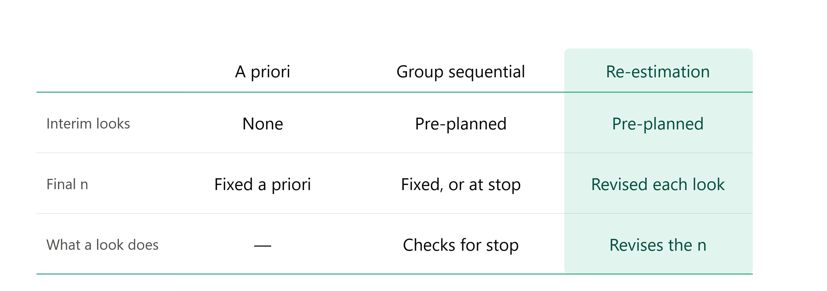
Comparison between a priori sample size estimation, group sequential designs, and sample size re-estimation

The most common way to plan a study is what is often called a priori planning: before the trial starts, you make your best guess about the effect size, calculate one sample size from it, and that is the number you aim to collect.

A group sequential design still starts from that same single guess. What it adds is a small number of pre-planned moments to look at the accumulating data and ask whether there is already enough evidence to stop, in either direction. If there isn’t, the trial continues toward the maximum sample size that was planned from the start.

NoteWhy not just look whenever?

You may have seen the word “pre-planned” in the column “Interim looks” in the table above. That means: a limited number of times and at a predefined moment (usually when the data of a predefined number of participants have become available). It might seem simpler to check the data informally, whenever it’s convenient, rather than committing in advance to a fixed number of looks. Two things go wrong with that. Look too early, and there usually isn’t enough data yet for the look to tell you much either way. Look too often, or without a plan, and each additional look becomes a fresh opportunity for random variation to look like real evidence purely by chance, so the overall false-positive rate creeps up well past the nominal one, even though each individual look still resembles an ordinary 5% test on its own. A trial can re-estimate more than once, at several pre-planned points in turn, but the same logic caps how many: each additional look has to be accounted for in advance, so the number stays small and fixed, not open-ended. Because looks are costly in this sense, deciding in advance how many times you’ll look, and when, matters as much as deciding what to do with what you see.

Sample size re-estimation also uses interim looks, but in a different way. Instead of only asking whether there is enough evidence to stop, at the interim you also recalculate the sample size using the current data, effectively setting the original guess aside, and revise the plan itself, including how many participants are still needed and, if relevant, when the remaining looks should happen. That is something a group sequential design does not do: its interim moments and final sample size stay exactly as pre-specified, however the data develop.

Suppose our trial follows part 1’s three-look schedule: interim analyses at 66 and 132 participants per group, with a planned maximum of 198. Say the interim at 132 participants suggests the effect is smaller than the original guess of 0.25. A group sequential design has nothing more to offer at that point: the trial either stops if the evidence already crosses the boundary, or continues to the fixed final look at 198, a number calculated under a guess the data no longer support. Sample size re-estimation lets you recompute instead. If the interim data point to 0.18, the new target of about 382 participants per group. Being able to revise recruitment plans for it during the trial may be worth a lot more than discovering it only once the originally planned 198 have already been reached.

When is sample size re-estimation especially useful?

Sample size re-estimation earns its value wherever the assumptions behind the original plan carry more uncertainty than a single a priori guess can really absorb. That uncertainty splits into two rather different issues: how sure you are about the parameters that go into the calculation, and how sure you are about the schedule built around them.

Uncertainty about parameters

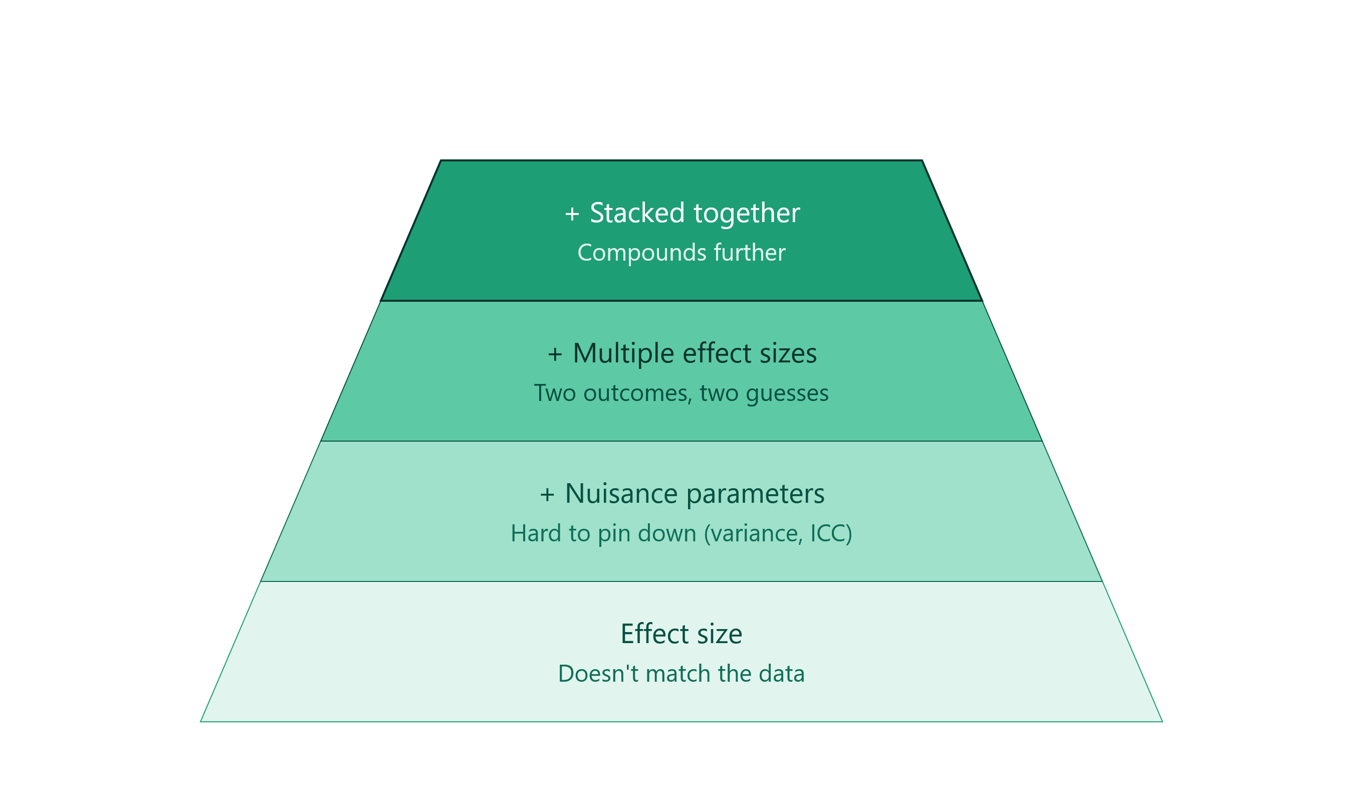
Cumulation of parameter uncertainty
  • The effect size itself. Guess it too optimistically, and the true effect turns out smaller: the trial ends up underpowered unless it can go beyond its pre-set maximum. Guess it too conservatively, and the true effect turns out larger: the trial collects more participants than it needed, though a group sequential design can at least partly correct for this by stopping early once the evidence is already strong enough. Sample size re-estimation’s particular advantage sits with the first case: it can raise the sample size when the data call for it, not only lower it through early stopping.
  • Nuisance parameters. Even a single effect size does not stand alone. In our original, single-outcome design, that parameter is the variance of body image scores. A pilot estimate can be off in either direction: too low, and the trial ends up underpowered because it assumed less spread in scores than there actually is; too high, and it enrolls more participants than needed. A different kind of nuisance parameter appears once the design changes shape. Suppose the trial recruited through several psychology practices rather than one, in effect turning it into a multilevel design, since participants are now nested within practices. Participants seen at the same practice tend to resemble each other somewhat, an intraclass correlation that depends on local factors like caseload and therapist style, and is rarely reported with much precision outside the specific setting it was measured in.

Assuming about 15 participants can realistically be recruited through each practice, moving the intraclass correlation from 0.10 to 0.30 raises what is needed from about 476 to about 1030 participants per arm, roughly 32 versus 69 practices, more than doubling the trial even though the effect size itself hasn’t changed at all.

A longitudinal version of the trial, measuring body image repeatedly over time instead of once at follow-up, introduces a related kind of parameter: how outcomes are expected to develop over time. That is another parameter that is difficult to point down, and also consequential for how many participants, and how many repeated measurements, the design actually needs.

  • Multiple parameters. Our trial in fact measures two outcomes, intuitive eating and body image. Planning for two outcomes means guessing two effect sizes correctly instead of one, which on its own already doubles the number of places the original plan can miss.
  • Multiple parameters and nuisance parameters together. In practice, multiple effect sizes rarely appear on their own: estimating two outcomes together also means assuming something about how they relate. Picture a version of our trial that is multivariate, multilevel, and longitudinal all at once: intuitive eating and body image, measured repeatedly over time, recruited through several practices. Planning that design means guessing two effect sizes, the correlation between the two outcomes, an intraclass correlation for participants nested within practices, and how each outcome develops over time. Every one of those numbers is a place the original plan can be wrong, and together they compound.

Uncertainty about the monitoring scheme

Parameter uncertainty rarely stays contained to the parameter itself. It carries over into the schedule built around it. Recall the pre-planned interim looks from part 1: 66, 132, and 198 participants per group, based on an assumed effect of 0.25. That schedule was built for that particular number. If the true effect were smaller, leading to a real requirement of around 382, the interim at 66 coul be too early to say anything useful about an effect that size, and by 132 you might still be well short. If instead the true effect only required around 140, stopping at 132, just short of enough, would be a frustrating near-miss. A schedule calibrated to one guess about the effect size is, almost by definition, miscalibrated for a different one.

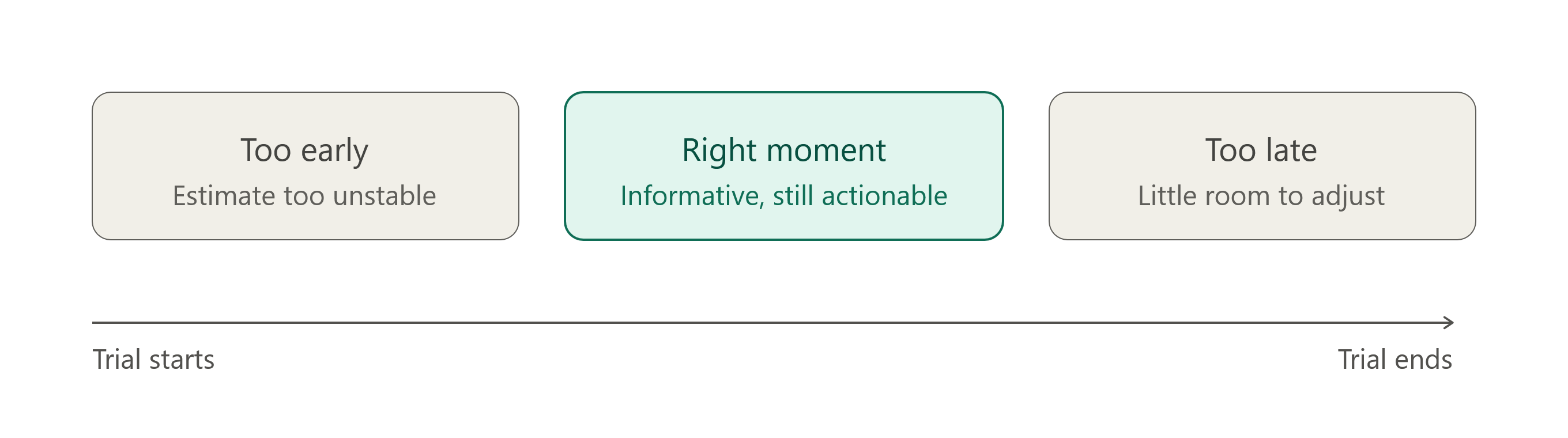
Timing of interim analysis matters

This points to a more general tension. Ideally, you want to look at the data, whether to re-estimate the sample size or to check whether a trial can already stop, at a moment when that look is genuinely informative. Too early, and the parameter estimate is still too unstable to trust, or the chance of stopping early is close to zero anyway, so the look adds little besides delay. Too late, and more data than a revised plan might have needed has already been committed, with limited room left to act on what you learn, on top of losing the practical benefit of knowing sooner how the rest of the study is likely to unfold. The two pulls do not always agree: what makes a look early enough to still act on can be exactly what makes it too early to trust. As early as possible, but as late as necessary, is the balance to aim for, and sample size re-estimation is what allows that balance to be revisited as the trial’s own data reveal more about where that point actually lies.

When does sample size re-estimation add less value?

None of this makes sample size re-estimation universally worthwhile. Its value tracks how much genuine uncertainty there is, and how much room there actually is to act on what an interim look shows. Both can be small enough that the effort buys little.

  • When the parameters are already reasonably well pinned down. A replication of our trial, run after the original has already produced a fairly precise effect estimate, has much less to gain from re-estimating: there is simply less uncertainty left to resolve. The same applies to a nuisance parameter like the intraclass correlation, if it happens to come from a setting that has been studied often enough to trust. This does not make sample size re-estimation pointless there, since some uncertainty almost always remains, but the expected gain is smaller, and the added complexity of an interim look may not be worth it for what is left to learn.
  • When the population is hard to reach and the maximum sample size is close to a hard ceiling anyway. If our trial recruited only through a handful of specialist practices for a rare presentation, there may be little practical room to expand recruitment even if an interim look suggested more participants would help. The stopping side of sample size re-estimation, ending the trial earlier if the evidence already justifies it, can still be useful here. The expanding side, raising the sample size beyond what was originally planned, is the part that loses most of its value.
  • When over- or under-shooting the original plan is genuinely low-stakes. If enrolling extra participants costs little in time, money, or burden, planning comfortably above the original guess and accepting some inefficiency if the effect turns out larger than expected may simply be easier than building in a formal re-estimation step.
  • When there isn’t a real opportunity to act on an interim look. This is less about the effect size and more about timing. In a longitudinal version of our trial, where body image and intuitive eating are measured well after enrollment, new participants can be enrolled faster than earlier participants’ outcomes become available. By the time an interim estimate is mature enough to trust, more participants may already be enrolled than a revised plan could still adjust for, even though the design looks sequential on paper. The “as early as possible, but as late as necessary” balance from the section above is what determines whether this is a real obstacle or just a scheduling detail to solve.
  • When the uncertainty itself makes a fixed number hard to work with. A defensible a priori estimate stays necessary either way: re-estimation can’t turn a trial capped at 100 participants into one that could handle actually needing 500. What it changes is how much weight that first guess has to carry, since it becomes a starting point data can correct rather than the one number everything rests on. Say the a priori estimate is 150, and even a pessimistic scenario puts the true number below 250: a practical maximum around there comfortably covers that range, and re-estimation can move freely within it. It works less well when the range is wider than that, say up to 400. A fixed ceiling of 250 doesn’t stretch to cover that, and no amount of re-estimation changes what the ceiling allows: the trial can find out sooner that it’s underpowered, but that isn’t the same as fixing it.

How does sample size re-estimation work, broadly speaking?

Show code
library(ggplot2)

nodes <- data.frame(
  id    = c("startbox", "interim", "check", "reest", "recalc", "another", "terminal"),
  x     = c(-6, 1, 8, 8, 8, 1, 15),
  y     = c(7, 7, 7, 3.8, 0.6, 0.6, 7),
  label = c(
    "Start data\ncollection",
    "1. Interim analysis\nreached",
    "2. Evidence to\nstop?",
    "3. Re-estimate\nparameters",
    "4. Recompute\nsample size",
    "5. Another interim\nplanned?",
    "Trial concludes\n(corrected for\nevery look)"
  ),
  type = c("start", "process", "decision", "process", "process", "decision", "final"),
  stringsAsFactors = FALSE
)

# Shrinks BOTH ends toward each other, for a segment that runs box -> box.
shrink_both <- function(x1, y1, x2, y2, margin) {
  dx <- x2 - x1; dy <- y2 - y1
  len <- sqrt(dx^2 + dy^2)
  frac <- margin / len
  data.frame(x = x1 + dx * frac, y = y1 + dy * frac,
             xend = x2 - dx * frac, yend = y2 - dy * frac)
}

# Shrinks only the START, for a segment leaving a box toward a plain waypoint
# (the waypoint end stays exact, so routing segments connect cleanly).
shrink_start <- function(x1, y1, x2, y2, margin) {
  dx <- x2 - x1; dy <- y2 - y1
  len <- sqrt(dx^2 + dy^2)
  frac <- margin / len
  data.frame(x = x1 + dx * frac, y = y1 + dy * frac, xend = x2, yend = y2)
}

# Shrinks only the END, for a segment leaving a plain waypoint toward a box
# (the waypoint start stays exact).
shrink_end <- function(x1, y1, x2, y2, margin) {
  dx <- x2 - x1; dy <- y2 - y1
  len <- sqrt(dx^2 + dy^2)
  frac <- margin / len
  data.frame(x = x1, y = y1, xend = x2 - dx * frac, yend = y2 - dy * frac)
}

h <- 2.4  # margin for horizontal arrows between two boxes
v <- 0.8  # margin for vertical arrows between two boxes

main_arrows <- rbind(
  shrink_both(-6, 7,   1, 7,   h),  # start -> interim (now same length as check -> terminal)
  shrink_both( 1, 7,   8, 7,   h),  # interim -> check
  shrink_both( 8, 7,  15, 7,   h),  # check -> terminal ("yes")
  shrink_both( 8, 7,   8, 3.8, v),  # check -> reest ("no")
  shrink_both( 8, 3.8, 8, 0.6, v),  # reest -> recalc
  shrink_both( 8, 0.6, 1, 0.6, h),  # recalc -> another
  shrink_both( 1, 0.6, 1, 7,   v)   # another -> interim ("yes")
)

# Exit route: another -> terminal ("no"), routed below steps 3 and 4.
# The waypoints at y = -2.0 are shared exactly between segments, so the dashed line stays continuous.
exit_route <- shrink_start(1, 0.6, 1, -2.0, v)                    # shrink near "another", waypoint exact
exit_turn  <- data.frame(x = 1, y = -2.0, xend = 15, yend = -2.0)  # waypoint to waypoint, no shrink
exit_final <- shrink_end(15, -2.0, 15, 7, v)                       # waypoint exact, shrink near "terminal"

labels_yn <- data.frame(
  x     = c(11.5, 8.9, 1.9, 1.9),
  y     = c(7.6, 5.4, 3.8, -0.7),
  label = c("yes", "no", "yes", "no")
)

type_fill <- c(start = "#9FE1CB", process = "#9FE1CB", decision = "#FCEFDC", final = "#E4DCF5")

ggplot() +
  geom_segment(data = main_arrows, aes(x = x, y = y, xend = xend, yend = yend),
               arrow = arrow(length = unit(0.3, "cm"), type = "closed"),
               color = "grey30", linewidth = 0.8) +
  geom_segment(data = exit_route, aes(x = x, y = y, xend = xend, yend = yend),
               color = "grey30", linewidth = 0.8, linetype = "dashed") +
  geom_segment(data = exit_turn, aes(x = x, y = y, xend = xend, yend = yend),
               color = "grey30", linewidth = 0.8, linetype = "dashed") +
  geom_segment(data = exit_final, aes(x = x, y = y, xend = xend, yend = yend),
               arrow = arrow(length = unit(0.3, "cm"), type = "closed"),
               color = "grey30", linewidth = 0.8, linetype = "dashed") +
  geom_label(data = nodes, aes(x = x, y = y, label = label, fill = type),
             color = "grey15", size = 4.2, fontface = "bold", lineheight = 0.95,
             label.padding = unit(0.5, "lines"), label.r = unit(0.35, "lines")) +
  geom_text(data = labels_yn, aes(x = x, y = y, label = label),
            size = 3.8, fontface = "bold.italic", color = "grey25") +
  scale_fill_manual(values = type_fill, guide = "none") +
  coord_fixed(xlim = c(-8.5, 17), ylim = c(-3, 9)) +
  theme_void()
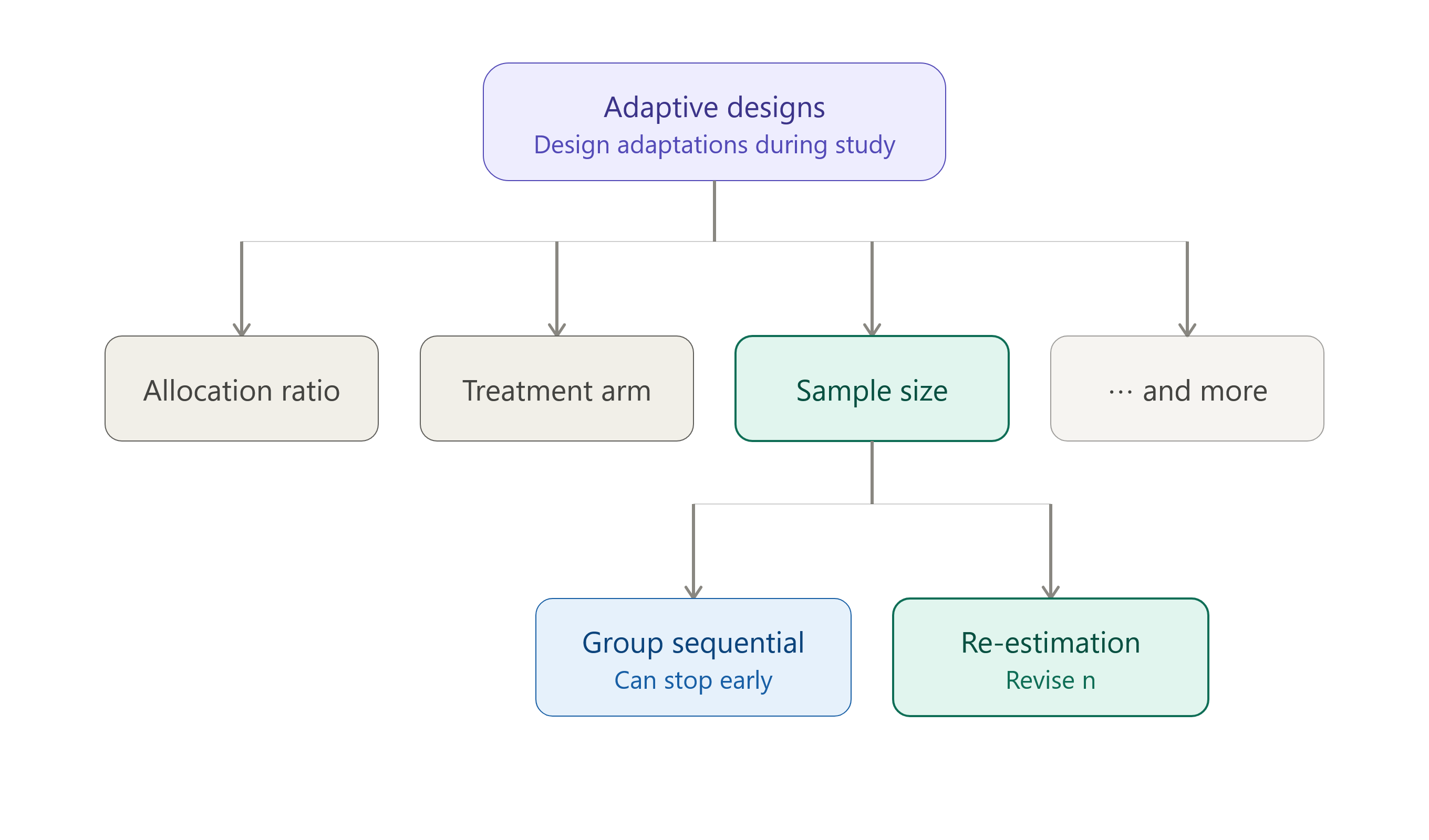
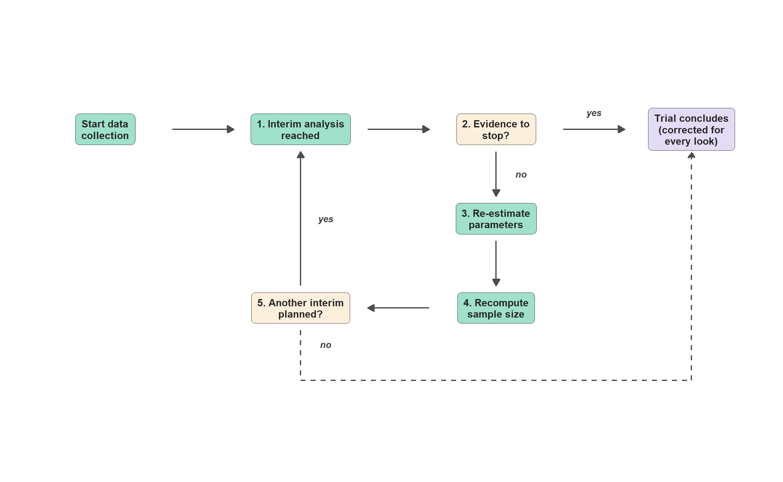
Figure 1: Sample size re-estimation
  1. Plan as usual, but build in the option to revise. Start with the best available estimate for every parameter the plan depends on, effect size and any nuisance parameters, and use it to set an initial sample size and monitoring schedule, exactly as any other design would. What’s different is deciding in advance that this plan is allowed to change, and specifying exactly when and how.
  2. Look at the accumulating data at a pre-planned moment. First check whether there is already enough evidence to stop, the same check a group sequential design would make. If not, re-estimate the parameters the plan depends on using the data collected so far. In our example, that means recalculating the effect on body image using the participants collected by then, rather than relying on the original guess of 0.25.
  3. Recompute what the trial actually needs. Using the updated estimates, redo the original sample size calculation, but now grounded in the trial’s own data instead of the literature. This can call for more participants, for fewer, or simply confirm that the original number still holds. Be aware: methods to re-estimate are usually different from the original computations, but that is beyond the scope of this blog.
  4. Update the plan, and either take another look or move to the final analysis. If another pre-planned interim remains, recruitment continues toward the revised target and step 2 repeats at the next look. Once no further interims are planned, the trial continues to the (possibly revised) sample size, and the eventual test is corrected for every look taken along the way, so that having looked more than once doesn’t inflate the false-positive rate.

Concluding remarks

Sample size re-estimation is best understood as a way of updating how much a trial commits to, using its own accumulating data, rather than staking everything on a single a priori guess. It helps most when there is real uncertainty to resolve, whether about the effect size, a nuisance parameter, several parameters at once, or the monitoring schedule built around them, and least when that uncertainty was already small to begin with, or when practical limits leave little room to act on what an interim look shows.

It is worth being honest about what re-estimation doesn’t do, too. It reduces uncertainty, but it never removes it entirely. If you already knew exactly what you would find at the moment of re-estimation or the moment of study termination, there would be no need to keep going, and no need for a trial at all. What sample size re-estimation offers instead is the chance to revise a plan once some of that uncertainty has resolved, using real data rather than an untested guess, while some uncertainty about the final answer necessarily remains until the trial actually ends. That is not a shortcoming specific to sample size re-estimation. It is simply what it means to design a study under uncertainty in the first place, which is exactly where this post started.

Questions? Any references that should be included as well? Found this useful? I’m on social media and happy to discuss!

Github BlueSky Mastodon LinkedIn ORCID ResearchGate
NoteA note on AI assistance

This post was developed in collaboration with Claude (Anthropic). Claude contributed to drafting and revising the text, and generated the R code used to produce the figures, based on an iterative exchange about content, framing, and design. The running example, the technical content, and all final editorial decisions are my own.

Citation

BibTeX citation:
@online{kavelaars2026,
  author = {Kavelaars, Xynthia},
  title = {Effect Size Uncertainty Is the Rule, Not the Exception -
    {Part} 2: {Sample} Size Re-Estimation},
  date = {2026-08-26},
  url = {https://xynthiakavelaars.github.io/OpenInferenceLab/posts/2026-08-sample-size-re-estimation/},
  langid = {en}
}
For attribution, please cite this work as:
Kavelaars, Xynthia. 2026. “Effect Size Uncertainty Is the Rule, Not the Exception - Part 2: Sample Size Re-Estimation.” August 26. https://xynthiakavelaars.github.io/OpenInferenceLab/posts/2026-08-sample-size-re-estimation/.